45 pivot table excel multiple row labels
How to set row limit in Excel - profitclaims.com #1 click the row 5 to select the entire row. #2 press Shift + Ctrl + Down Arrow keys in your keyboard, to select all rows from row 5 to the bottom of the worksheet. #3 right click on the selected rows and choose Hide from the popup menu list. #4 click on the Column D to select the entire column. powerspreadsheets.com › excel-pivot-table-groupExcel Pivot Table Group: Step-By-Step Tutorial To Group Or ... In fact, as mentioned in Excel 2016 Pivot Table Data Crunching: Each time you create a new pivot table in Excel 2016, Excel automatically shares the pivot cache. Pivot Cache sharing has several benefits. Most notably, as I mention above, it reduces memory requirements and file size vs. the scenario where the Pivot Cache isn't shared.
stackoverflow.com › questions › 55735003Excel Pivot Table with multiple columns of data and each data ... Apr 17, 2019 · Then I made multiple Pivot Tables, filling the Columns and Values Pivot Table Fields with one Category of each of your categories. This will produce a Pivot Table with 3 rows. The first row will read Column Labels with a filter dropdown. The second row will read all the possible values of the column.
Pivot table excel multiple row labels
How to Create a Swimlane Flowchart in Excel (With Easy Steps) Right-click on the selected rows. Then, click on the option Row Height. Furthermore, set the value 50 in the Row height input field. Now click on OK. Next, select cell ( B5:B8 ). Moreover, go to the Home tab. Click on the Borders icon, and select All Borders from the drop-down menu. After that, select cells ( C5:L8 ). › excel-pivot-table-formatHow to Format Excel Pivot Table - Contextures Excel Tips May 23, 2022 · Keep Formatting in Excel Pivot Table. A pivot table is automatically formatted with a default style when you create it, and you can select a different style later, or add your own formatting. For example, in the pivot table shown below, colour has been added to the subtotal rows, and column B is narrow. excel - Incorrect Calculations in Pivot table when adding a measure ... Incorrect Calculations in Pivot table when adding a measure. I have made a pivot table of data in which there is a row label and two columns - sum of amount and sum of the actual cost of units, also I have added a measure (profit) which has the formula of subtraction between two sums column. After adding the profit measure to the pivot table ...
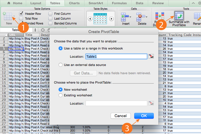
Pivot table excel multiple row labels. datagy.io • datagy Welcome to datagy.io. Learning data science can be hard. It can be frustrating. It can also be confusing. That's where we come in - datagy is a site that makes learning different data science and Python skills intuitive and easy to understand. Our in-depth guides often provide more than a handful of different ways to be able to accomplish ... › xlpivot08Excel Pivot Table Multiple Consolidation Ranges Nov 15, 2021 · Pivot Table from Multiple Consolidation Ranges To open the PivotTable and PivotChart Wizard, select any cell on a worksheet, then press Alt+D, then press P. That shortcut is used because in older versions of Excel, the wizard was listed on the D ata menu, as the P ivotTable and PivotChart Report command. Excel Worksheet Printing Tips 🖨️ Printing Problem Fixes On the Ribbon, click the Page Layout tab, and click Print Titles In the Page Setup window, on the Sheet tab, click in the Rows to Repeat at Top box. On the worksheet, select the row (s) that you want to print at the top of each page. The row numbers will appear in the Page Setup window. Click OK, to close the window. Rows to Repeat Not Available How to Reverse Order of Columns Horizontally in Excel =INDEX ($B$5:$C$8,ROWS (B5:$B$8),COLUMNS ($B$5:B5)) Then, press Enter on the keyboard. Drag the Fill Handle down to duplicate the formula over the range. Or, to AutoFill the range, double-click on the Plus ( +) symbol. Further, to replicate the formula throughout the range, drag the Fill Handle rightwards.
Import data from Excel to SQL - SQL Server | Microsoft Docs The Import Flat File Wizard. Import data saved as text files by stepping through the pages of the Import Flat File Wizard. As described previously in the Prerequisite section, you have to export your Excel data as text before you can use the Import Flat File Wizard to import it.. For more info about the Import Flat File Wizard, see Import Flat File to SQL Wizard. › excel › indexExcel Pivot Table Report - Clear All, Remove Filters, Select ... Excel Pivot Table Report - Clear All, Remove Filters, Select Mutliple Cells or Items, Move a Pivot Table. As applicable to Excel 2007 With the tools available in the Actions group of the 'Options' tab (under the 'Pivot Table Tools' tab on the ribbon), you can Clear a Pivot Table, Remove Filters, Select Multiple Cells or Items, and Move a Pivot Table report. Tutorial: From Excel workbook to stunning report in Power BI Desktop ... In the Fields pane on the right, you see the fields in the data model you created. Let's build the final report, one visual at a time. Visual 1: Add a title On the Insert ribbon, select Text Box. Type "Executive Summary - Finance Report". Select the text you typed. Set the font size to 20 and bold. Resize the box to fit on one line. CONCATENATEX - DAX Guide This article describes how to correctly use column references when manipulating tables assigned to DAX variables, avoiding syntax errors and making the code easier to read and maintain. » Read more. This article showcases the use of CONCATENATEX, a handy DAX function to return a list of values in a measure.
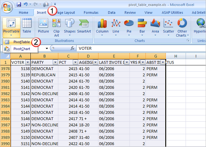
How to Add Calculated Field to Pivot Table in Excel - Sheetaki The Pivot Table below uses the Country field as a row label. In column C, we've added a calculated field that deducts a certain percentage from the sum of all sales in a particular country. To get the values in Column C, we just need to use the following formula: = total_sales - (total_sales * 12%) en.wikipedia.org › wiki › Pivot_tablePivot table - Wikipedia Pivot tables are not created automatically. For example, in Microsoft Excel one must first select the entire data in the original table and then go to the Insert tab and select "Pivot Table" (or "Pivot Chart"). The user then has the option of either inserting the pivot table into an existing sheet or creating a new sheet to house the pivot table. Headers Sheets Multiple With In How Same To Vba Merge Excel hold down ctrl and then left click the mouse on each worksheet tab in column c, type the following excel formula and your command is ready to be executed then, switch to the workbook that you want to copy several sheets from insert a module in vba editor and copy above vba code a box at a particular column and row is called a cell a box at a … How to Reduce Decimals in Excel - Sheetaki How to Add Calculated Field to Pivot Table in Excel You May Also Like Read More. M ... March 22, 2022; This guide will show you how you can convert multiple rows to columns and columns to rows in… Read More. M Microsoft Excel. How to Find Circular References in Excel. by ... How to Add Axis Label to Chart in Excel. by Aimee Alvarez; May 25, 2022;
How to Create a Pivot Table in Excel: A Step-by-Step Tutorial (With Video)
Excel Fiscal Year Calculations and Formula Examples Calculate the Fiscal Year. Based on the month number in which the fiscal year starts, you can use the IF function to calculate the fiscal year for any date. In this example, the starting month is entered in cell C4, and the date is entered in cell C6. The following formula is entered in cell C8:

Grouping Dates in Pivot Tables - Show Pivot Reports by Month, Quarter, Week or Hour of Day ...
Basic Excel Tutorial Excel can be used with text data apart from numerical data. You could use it to record a business's names, goods, or services. The test data should be made by capitalizing the first letters of all the words in the cells. You may want to capitalize the first letter of each word or only the …. Read more.

How to Sort Pivot Table Row Labels, Column Field Labels and Data Values with Excel VBA Macro ...
excel.officetuts.net › examples › filter-multipleHow to Filter Multiple Values in Pivot Table – Excel Tutorials Our Pivot Table now looks like this: Filter with Pivot Table Label Filters. Now we will clear all of our filters. To clear them all out at the same time, we will click anywhere on our Pivot Table, then go to PivotTable Analyze field >> Actions >> Clear Filters: Once we do that, we will go to our Pivot Table, go to a dropdown at the Row Labels ...

Split data into multiple tabs from pivot table - Excel Launchpad
EOF

Excel Pivot Table Tutorial & Sample | Productivity Portfolio
Mail Merge Multiple Rows Into One Document :: blogshoe54 Start the Mail Merge Wizard. For this, go to the Mailings tab, and click Start Mail Merge > Step-by-Step Mail Merge Wizard. The Mail Merge panel will open on the right side of your document. In step 1, you choose the document type, which is E-mail messages, and then click Next to continue.

Excel-VBA-Macros-SQL-Examples-Tutorials-Free Downloads: How to Sort Pivot Table Row Labels ...
Apply dependent combo box selections to a filter - Get Digital Help Press CTRL + SHIFT + ENTER. Copy cell B2 and paste it down as far as needed. The values in column B change depending on selected value in the combo box on sheet "Filter".

30 Using The Current Worksheets Pivot Table Add The Task Name As A Column Label - Labels For You
How to use VLOOKUP with multiple conditions - Get Digital Help Use the table name and table column name in the VLOOKUP function to achieve this, see the formula bar in the picture above. How to convert a cell range to an Excel defined Table? Select any cell in your data set. Go to tab "Insert" on the ribbon. Press with left mouse button on "Table" button to open a dialog box. Enable "My table has headers".

How to Sort Data in a Pivot Table | Excelchat
Excel Row Start Laravel - pws.taxi.veneto.it Search: Laravel Excel Start Row. Once the first row is given, we can just add the total rows in the range and subtract 1 to get the last row number A single cell or range of cells, you may have to be returned to the number of rows and number of columns, can be specified {{ __('авторизоваться') }} Здравствуйте, я создаю мультиязычный сайт In ...

Excel Pivot Table Report - Sort Data in Row & Column Labels & in Values Area, use Custom Lists
excel - Incorrect Calculations in Pivot table when adding a measure ... Incorrect Calculations in Pivot table when adding a measure. I have made a pivot table of data in which there is a row label and two columns - sum of amount and sum of the actual cost of units, also I have added a measure (profit) which has the formula of subtraction between two sums column. After adding the profit measure to the pivot table ...
Excel Pivot Table Tutorial & Sample | Productivity Portfolio
› excel-pivot-table-formatHow to Format Excel Pivot Table - Contextures Excel Tips May 23, 2022 · Keep Formatting in Excel Pivot Table. A pivot table is automatically formatted with a default style when you create it, and you can select a different style later, or add your own formatting. For example, in the pivot table shown below, colour has been added to the subtotal rows, and column B is narrow.

Repeat Pivot Table row labels • AuditExcel.co.za Pivot Tables Course
How to Create a Swimlane Flowchart in Excel (With Easy Steps) Right-click on the selected rows. Then, click on the option Row Height. Furthermore, set the value 50 in the Row height input field. Now click on OK. Next, select cell ( B5:B8 ). Moreover, go to the Home tab. Click on the Borders icon, and select All Borders from the drop-down menu. After that, select cells ( C5:L8 ).
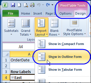
Repeat Pivot Table Labels in Excel 2010 - Excel Pivot TablesExcel Pivot Tables
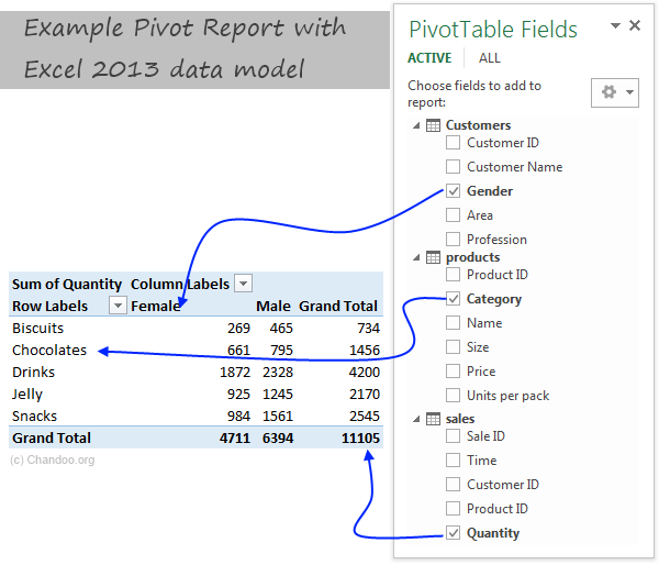
Introduction to Excel 2013 Data Model & Relationships » Chandoo.org - Learn Excel, Power BI ...

Excel Pivot Table Defaults - Changing Layout, Repeating Labels, and Subtotals - YouTube
multiple fields as row labels on the same level in pivot table Excel - Microsoft Community

33 Pivot Table Blank Row Label - Labels Database 2020
Post a Comment for "45 pivot table excel multiple row labels"